Lab 6: GIS Analysis of Slope
Katie Burles and Crystal Huscroft
In this lab you will be doing an office-based analyses of topographic slope.
Slope is a measure of change in elevation over a known horizontal distance. Often it is used to describe the steepness of a landform surface. One might argue that slope is one of the most significant landscape metrics for geographers to evaluate.
Much of Earth’s surface is sloping, not flat, and as a consequence there are a range of hydrological and geotechnical processes that are activated by the difference in potential energy between one location and another. Potential energy is the energy available to for doing work. For example, an object that is lifted above Earth’s surface to height H can be moved downward a distance H by gravity. Slope processes bridge several scientific fields such as geomorphology, soil science, hydrology, and engineering.
In this lab, using a Geographic Information System (GIS), you will measure the gradient of a ski run at a resort of your choosing, plot the vertical profile and produce a short report summarizing your findings.
Learning Objectives
After completion of this lab, you will be able to
- Measure elevation and distance using online GIS platforms.
- Calculate slope gradient using a spreadsheet program.
- Generate slope profiles using a spreadsheet program.
- Relate field observations of gradient to calculated values of gradient.
Pre-readings
Contour Lines
Contour lines (or simply contours) on a topographic map are the most common way of showing the three-dimensional landscape. With practice, a geographer can easily visualize the landscape from a two-dimensional map sheet—a valuable skill.
Contours are lines that connect points of equal elevation. One way of envisaging this is to imagine a valley filled with water. If you drew a line along the shoreline, it would be a contour line. If you dropped the lake level by, say, ten metres and again drew a line along the shoreline you would have a second contour line. Repeating this exercise again and again would leave you with a landscape covered in horizontal lines all ten vertical metres apart (known as the contour interval). You have just made a topographic map! In practice, contours are typically derived by a combination of ground surveys and analyses of aerial photographs.
If we follow the hypothetical procedure for deriving 10-metre contours outlined above, it will be obvious that in very flat areas, a contour interval of ten metres will probably not allow you to pick up the subtleties of the landscape. On the other hand, in a mountainous region a contour interval much greater than ten metres would be advisable, otherwise there would be so many contours that nothing else could be mapped! So, always check the contour interval of the topographic map you’re using. It will normally be found in the map’s legend. You will also normally find that contour interval increases as map scale decreases.
A map’s contours allow us to derive some fundamental pieces of information: how high we are (our elevation), the steepness (or gradient) of the slope, the slope’s profile shape, and the overall relief of the landscape.
Types of Contours
There are several different types of contours that are good to know about:
- Index contours. Typically, every fifth contour is a bolder line than the regular contour. This is especially useful in high-relief terrain because it allows us to find elevations from the map without having to count every single contour: we can go up/down the mountainside by jumping from one index contour to the next.
- Approximate contours. These are similar to regular and index contours but are drawn using a short-dashed line. This indicates that the exact elevation of the surface was difficult to determine and/or may vary in time.
- Auxiliary contours. If a map shows low-relief terrain adjacent to high-relief terrain, extra contours with a smaller contour interval are sometimes used in the low-relief area to provide more topographic detail. On NTS maps, these are depicted as long-dashed brown lines.
- Depression contours. (Figure 6.1a) These indicate where the land inside a closed-loop contour is lower (i.e., a depression – or hollow – in the surface). The contour line has small hachure marks that face downhill, into the depression.
- Cliff symbol. (Figure 6.1b) Okay, so this is not an actual contour line, but it is worth adding to our list. When slopes get very steep and become cliffs, it may be difficult or impossible to use contours, so a symbol is used instead. The tightly-spaced hachure marks indicate the way the cliff faces.

Interpreting Contour Lines
When interpreting contour lines, there are several key points to remember:
- A contour always separates land that is higher from land that is lower.
- All contours are single, continuous lines. They do not split or cross over each other.
- A closed-loop contour always indicates that there’s higher ground inside the loop, unless it is a depression contour.
- On Canadian NTS maps, the convention is that contour labels are oriented to indicate which is uphill. Look carefully at Figure 6.2, for example: along the Illecillewaet River valley at the bottom of the figure, you can see two contour labels on either side of the valley, 3800 and 4200. Uphill is the direction above the top of the number if you were reading it normally.
- If you see contours form a V pattern along a watercourse, the V always points upstream. If you’re at a sharp ridge, such as a glacial arete or a large lateral moraine for example, the V pattern in the contours points downhill. Figure 6.2 has several good examples: note the contours along Cougar Brook (at the bottom SW of the figure) where the V pattern points uphill, toward the creek’s headwaters. Just to the east of there, examine the contours at Napoleon Spur – the V pattern points down the ridge crest.
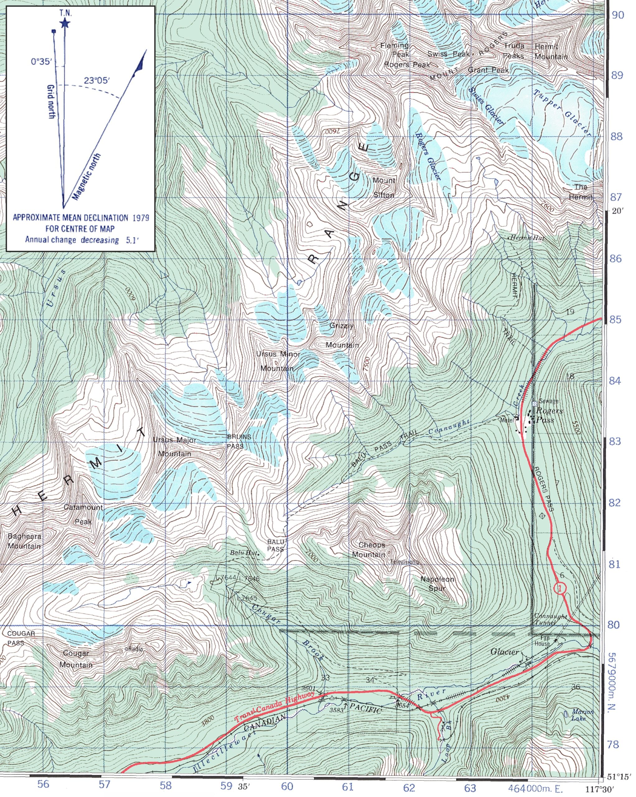 Figure 6.2. Part of NTS 1:50,000 map sheet 82N05 (Glacier) 3rd edition. Elevation units are in feet. Magnetic declination is 22°30′ E. Grid declination is 23°05′ E. Grid convergence angle is 35′ W. The grid declination is decreasing 5.1′ annually. Source: Natural Resources Canada, Open Government License-Canada.
Deriving Slope Gradients from Maps
There are several different ways of expressing slope gradient, and all of the most common ones are based on the ratio of horizontal and vertical distances between two points (the classic rise over run situation). To find the slope we need two values: the horizontal distance between points A and B, and the elevation difference between them (Figure 6.3). The horizontal distance (Δx) is found by measuring it on the map and using the map’s scale to convert to real-world distance . The vertical distance between A and B (Δz) is the elevation difference between them, which can be found by interpolating from contours and/or spot heights.
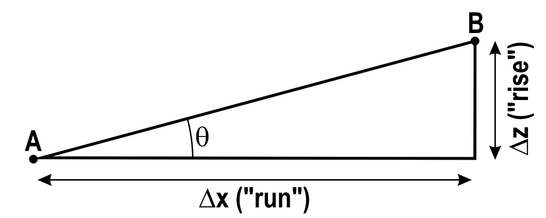
Once we have this information, the slope gradient can be calculated and expressed in three ways:
- As a percent (%): the fraction (rise ÷ run) expressed as a percentage (Equation 6.1):
- As an angle, θ (degrees) (Equation 15.2):
- In elevation change per slope distance (m/km): the gradient expressed with different units used for rise and run, but with the run always reduced to one unit, commonly 1 km (Equation 6.3):
For example, let us assume that the elevation difference we interpolated between points A and B from contour intervals is 70 m, and the distance measured between A and B is 560m after converting with the map scale. Using the equations presented above, we can express our slope gradient as
- As a percent (%) (Equation 6.1):
- As an angle, θ (degrees) (Equation 6.2):
- In elevation change per slope distance (m/km) (Equation 6.3):
If you don’t have a calculator with trigonometric functions, you can use an online Arctan Calculator to find the inverse tangent. You will need to divide the rise by the run (70560) as an input for this particular calculator.
Notice that in Figure 6.8 the horizontal distance separating A and B (i.e. Δx) is not the actual ground distance. The true distance from A to B is along the hypotenuse of the triangle in Figure 6.8. For small slope gradients the difference between A-B distance and Δx is negligible, but in steep terrain the A-B distance will be significantly longer than Δx.
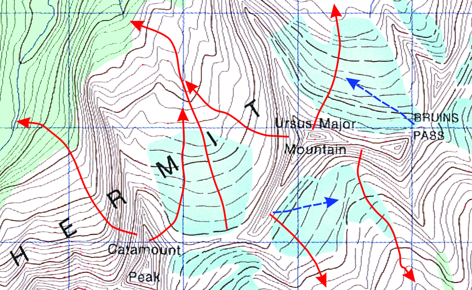
Finally, when deriving slope steepness from a map you must measure Δx along a line that is perpendicular to the contours. This gives the true slope, equivalent to the fall line – think of the direction that water would run down a slope: it would move down the steepest, most direct path, and not deviate along lower-angled routes. In Figure 6.3, true slopes are shown with red arrows. Notice how the red arrows cut across contours at a 90º angle. All other lines crossing the contours represent a false slope (blue arrows), which will always be less than the true slope. On simple slopes, you may be able to measure Δx along a straight line, but realise that the line of true slope will often be curved, as in Figure 6.3.
Topographic Profiles
A topographic profile (Figure 6.4) is a cross-sectional diagram through the landscape, which helps us envisage the nature of the terrain. A profile line might be a simple straight line (which generates a simple profile), or a series of straight lines connected at angles to each other (which generates a compound profile), or more or less any other continuous line, straight or curved. If we used a profile line that cross all of the contours at right-angles, we would have a transverse profile. The longitudinal profile of a river is a transverse profile familiar to geomorphologists and hydrologists.

Topographic profiles are commonly employed to simply show the ups and downs along a particular line (often used in depicting the slopes along a hiking trail). They may also be a bit more complicated like a cross section and show the subsurface geology, such as the way rock strata tilt and/or fold beneath Earth’s surface.
It is common to find that topographic profiles are vertically exaggerated (stretched in the vertical direction) to better depict the subtleties of the terrain. Vertical exaggerations of up to about 3x are common; anything more than this tends to make every little bump in the landscape look like hills and mountains!
Lab Exercises
This lab results in creating an assignment to be handed in as a report in PDF format. The submitted report will include a series of required figures with captions.
This exercise is office-based and will take approximately 3 hours to complete if you attend lab Face 2 Face. Although, the length of time allocated to this exercise will depend on familiarity using Google My Maps, iMapBC, and Microsoft Excel.
Required software:
- iMap BC website (no user name required).
EX2: Create a Slope Profile of a Ski Run at a Ski Hill in British Columbia
Step 1: Choose a Ski Run
Open Google My Maps. Click Create a new map. Using the search function on the left of your screen, visit a ski hill (resort) in British Columbia. The BC Ski Map contains more information about BC ski resorts. Zoom into the ski hill until all the lifts and runs are visible on the map. Select one ski run to use in this exercise.
It is recommended that you select a ski run below treeline which is easily traceable on satellite imagery. Ski runs should be longer in length, as short ski runs have few slope breaks. The ski runs at some smaller ski resorts may not be available on Google My Maps.
Post your chosen ski run on your class’s wiki (see Moodle).
Step 2: Outline the Ski Run Using Google My Maps (Figure EX2.1)
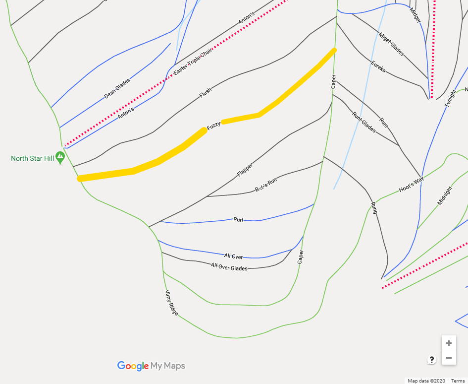
Select Add layer and draw a thick yellow line over the ski run selected (see example Figure 6.10). Include a screen capture of the run with the name visible in this exercise. Add marker adjacent to the bottom of the ski run and record the latitude and longitude of this location in decimal degrees. Share the Layer and copy the link to include in the Figure EX2.1 caption. Your caption should also include a description including the ski hill name and coordinates.
Step 3: Draw and Describe the Profile of the Ski Run Using iMapBC (Figure EX2.2)
Open iMapBC and launch application (Launch iMapBC). Select the option that does not require a username. Change the base map from Roads to Imagery. The icon is located in the bottom-left of the screen. The ski hill lifts and runs are not drawn in iMapBC, but they are visible as clear-cut areas in the imagery.
Find your ski run. Using the Lat/Long function in the tool bar, zoom to the run. To input Lat/Long, convert the units from decimal degrees to degrees, minutes, and seconds. Use the National Geodetic Survey Coordinate Conversion and Transformation Tool to convert. Input the Lat/Long in degrees, minutes, and seconds to zoom into the ski run in iMapBC.
Add Provincial Layers on the Go to Data Sources tab. Search layer catalog for Contours – (1:20,000) (Base Maps – Contours – Contours – (1:20,000)).
Create Figure EX2.2 for your report by drawing the ski run using the tools on the Sketch tab. Using the Edit tool, change the Styles of the line to change the colour and pattern of the line. Using the Identify tool on the Home tab, find the maximum and minimum elevation of the ski run. Using the Distance tool on the Sketch tab, measure the length of the ski run. Add Text to the map on the Sketch tab, including the name of the run, the run length (e.g., Run = 832.3 m), and the maximum and minimum elevation (see example Figure 6.11). Take a screenshot of the image.
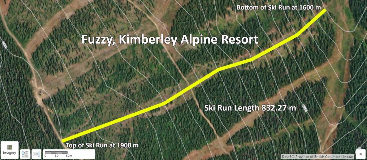
Step 4: Describe the Natural Breaks in Slope for the Ski Run (Figure EX2.3 and Table EX2.1)
By inspecting changes in the spacing of contour lines along the path of the run, divide the ski run into 4 segments at natural breaks in slope. Breaks in slope indicate a change in physical continuity in the slope profile. Segments of your ski run may be steeper (more linear distance between contour lines closer together) than other sections.
Position your breaks in slope where your path (the ski run) crosses a contour line. Measure the horizontal distance between each slope break segment and record the elevation. This will be Figure EX2.3 in your report. Figure 6.12 is an example outlining four slope break segments selected for the Fuzzy ski run.
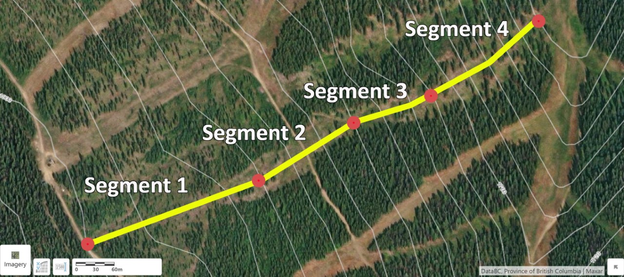
Create Table EX2.1 in your report to include the measurements you collected. An example is provided as Table 6.3.
Step 5: Create a Profile in Microsoft Excel (Figure EX2.4)
Open Microsoft Excel and enter the data in columns similar to Table EX2.1 (Table 6.3). Figure EX2.4 in your report will be a profile of the slope using a Scatter (x.y) Chart (see example Figure 6.13, Example Figure 6.13 [Excel]).
Do not plot from sea level (0 m). Adjust the maximum and minimum values displayed on the ski run elevation axis (y) to optimize the range of elevation in the profile. For example, the y axis in Figure 6.13 ranges from 1550 m to 1950 m. Microsoft Excel will default the axis to start at 0 m.
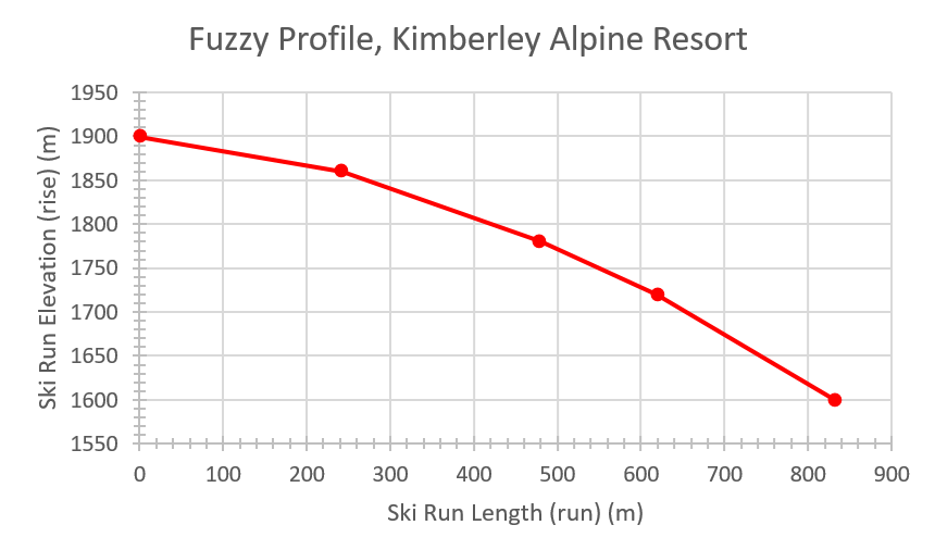
Step 6: Calculate Gradient Using Microsoft Excel
Calculate the slope gradient in Excel using the three calculations provided in Calculating Slope Gradient. Calculating gradient in degrees in Excel requires the use of the =ATAN function. The complete Excel expression is =(ATAN(rise/run)*(180/PI())). ATAN is an abbreviation for arctan, which is denoted tan-1. PI() is the notation for π in Excel.
Calculate the average gradient for each segment and include in Table EX2.2. An example is provided as Table 6.4.
Step 7: Assemble EX2 Component of Your Lab Report
Open the Word document created in EX1. Add EX2 and include Figures EX2.1 to EX2.4 and Tables EX2.1 and EX2.2 with detailed captions for each. Table 6.5 provides a checklist.
| Item | Description | Caption (Attribution) |
| Figure EX2.1 | Google My Maps screen capture of the ski run. | See example Figure 6.10 (Image Source – Google My Maps Attribution). |
| Figure EX2.2 | iMapBC screen capture of the ski run including the name of the run, 20 m contour lines, maximum and minimum elevations, and run length. | See example Figure 6.11 (Image Source – iMapBC Attribution). |
| Figure EX2.3 | iMapBC screen capture of the 4 natural slope breaks you used for your profile. | See example Figure 6.12 (Image Source – iMapBC Attribution). |
| Table EX2.1 | Data collected for the 4 natural slope breaks you used for your profile. | See example Table 6.3. |
| Figure EX2.4 | Profile of your ski run created in Microsoft Excel. | See example Figure 6.13. |
| Table EX2.2 | Gradient calculations completed in Microsoft Excel for your ski run, including average slope. | See example Table 6.4. |
Reflection Questions
Please take 15 minutes to answer the following questions using the experiences gained in completing this lab and from this course in general. Limit your answers to a maximum of 150 words.
EX2
- In your own words, what skills did you gain in this lab?
Create a new part of your lab assignment titled Reflection Questions and type in your answers.
Report Submission
Once all exercises are complete, save the assignment as a PDF and submit as directed by your instructor. The PDF submission should be saved in Layout – Orientation – Landscape with images taking up at least 75% of the area of the page.
Supporting Material
References
Mulu, Y.A., Derib, S.D, 2019. Positional Accuracy Evaluation of Google Earth in Addis Ababa, Ethiopia Artificial Satellites 54(2).

